This was an undergraduate computer vision extra-curricular project.
Image segmentation goal: finding text within am image of a road sign
The growing abilities of video feed APIs allow for mobile and domain-specific programs that were previously out of reach. One application that I had in mind was video frame text extraction, which itself could be the foundation for magnification or text-to-speech capability that could aid the visually impaired, translation for foreign language signs and contextual advertising services. The idea is to help foreigners understand local signs.
Update: Since this article was written, Google Goggles has been released and implements much of the functionality described here
Of course I can’t do all of this alone; so the goal I’d set out to meet was simple: develop an algorithm for text detection using a Multi-layered Perceptron Neural Network (feed-forward neural network). In addition, the entirety of the implementation was to serve as an easily- modified and reusable scaffold for further experiments in neural networks.
Approach
In creating the dataset (both training and test), Google Image Search returned 30 photos of street signs. I then wrote a markup- generator to mark which areas contained text as part of the supervised training. The “correct” regions are highlighted and these are used later to check if the neural network predicted correctly. The overlay is a simple bitmap: non-zero alpha bit for the text areas and zero alpha otherwise. All 30 images are marked by highlighting the regions and saving the highlighting overlay.
Since many of the images contained extremely high levels of noise in both the compression format as well as through non-important textures, a Gaussian blur had to be run twice through each tile of the image before being fed into the sensitive edge-detection and energy filters.
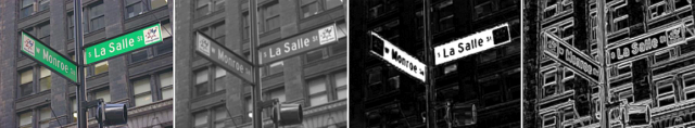
The Energy filter was created empirically after much experimentation. Visually, I played around with various schemes of luminance and displayed the result in the runFilters code that was written until a satisfactory contrast detection filter was had. EnergyMap is particularly sensitive to road signs. The Sobel operator was found through literature and applied in its 3x3 configuration.
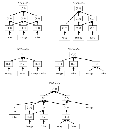
Several different neural network layouts were tried. Each one was trained by breaking the image into 8x8 tiles, feeding those tiles through a few filters and then through the nodes of each NN. You can see the schemes for several of the NNs, as well as the object design, in the code below:
Implementation
The complete NN framework (supervised training set generator, NN training program, NN test program) was written from scratch in JavaScript for maximum portability, allowing users to run the software from any computer with a modern web-browser. Internet Explorer is not supported due to lack of support for the canvas tag.
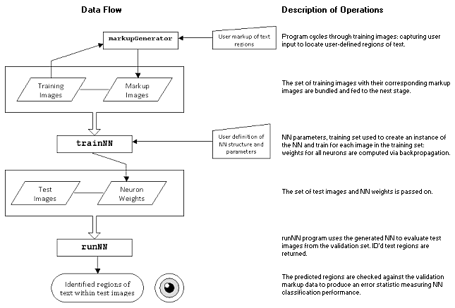
The first step in implementation was to feed a set images and a markup of the text regions on those images. These two sets were then used in determining the weights for the nodes of our models. Our test set consisted of 3 images that were part of the original validation set, this is because the correct areas are already marked so testing the NN could be done automatically. Below is a system schema.
The chosen activation functions between the Neurons in the NN should be sigmoid functions as is standard with references. Due to this fact, backpropagation with the delta rule, for output layer neurons, of which there are exactly 1 in each model, becomes:
Delta output = (actual output)(1 - actual output)(desired output - actual output)
Deriving the derivative for the sigmoid function via chain rule, we get the delta rule for the hidden Neurons:
Delta hidden = (actual output)(1 - actual output)( Sum(delta receiver neuron) dot product W receiver neuron for hidden)
These delta values are used in conjunction with the learning rate and the momentum of weight change parameter to change the weights with each backpropagation. A typical sequence for a single 8x8 tile requires that we activate the NN first and then backpropagate the errors through the NN to correct for mistakes in classification.
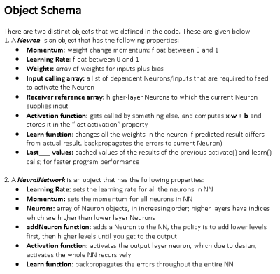
To build layers, we create the individual neurons and then link them together in the input calling
arrays for each layer, as well as through the receiver arrays. The NN creation code can be seen in NN.js.
This way, the network can be arbitrarily arranged and we can have skip-layer connections from one level to
any higher level.
Initial Model Parameters
Determining the threshold of the output layers proved to be an immense challenge. There is no standard way of solving this optimization problem so with the limited time we had to finish this project we tried many thresholds through trial and error. Given more time, we would probably implement an automatic cross-validation system that would give better estimates on a suitable threshold.
To be on the safe side, our implementation of the threshold estimate was highly lenient and rounded down to the first significant digit minus 1 (0.033 ~ 0.02). To get this number, we gathered the total output values for correct and incorrectly predicted tiles and then took the normal and geometric mean of the two. Roughly our threshold formula is:
t NN = Ugm - | Ugm - Um |

Threshold NN = (Floor( 100 t NN ) - 1) / 100
This works well enough as a starting point and was already a better threshold. Eventually through manual cross-validation in Excel we reached a threshold of 0.02144445 which gave us the best threshold for the NN1 model. Thresholds for other models were obtained in a similar fashion.
Model Performance
The models were evaluated using misclassification rate on the regions returned as text for the images. Defining what constitutes as false positive and as false negative was a bit of a challenge. As a case in point, borders of signs which also had high energy gradient and similar colour and style as the text they enclose could be argued as being text or not. We made these assumptions in determining the misclassification rate:
- Small text or illegible text that were not detected were classified as true negative
- Borders detected as text will be classified as false positive
- Other non-marked areas will be classified as true negative
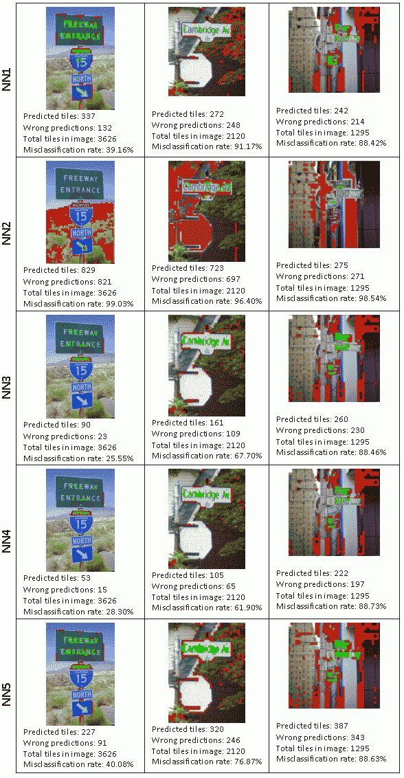
This was consistent with our markup images and thus the test set used in the runNN program gave us the misclassification rates. Red tiles are predicted tiles which were incorrect, green tiles are predicted tiles which are confirmed correct with our markup validation data. These are the results of each model being run on the test set:
In short
We found that several factors influenced the ability to detect text. Some of the more obvious ones include font size and colour of the text, amount of lighting in the picture, and even the texture and complexity of the background. First off, our definition of what text was appeared to cause a lot of errors in the generated model. We did not tightly control what passed for a “text region” other than a qualitative sense of whether or not the region was legible. This would have had a major impact on our selection for training images and markup. If we had used only a certain size font as the training set target then perhaps a better result could be obtained. This same problem exists in the test set as it was part of our data set that we had gathered.
Our training set could have also been much greater for the more complex models such as NN1 and NN2. No doubt the ambiguities would have been less severe in swaying the classification of models of greater layers. Furthermore, the parameters for the models raise questions about how they might be changed or determined to a precision. Without a good threshold it is very hard to isolate the good classifications from the false ones.
The generated system produced some reasonable results, an improved version could be well used as the basis for a separate feature extraction or classification system. It could also be improved if more edge features and image processing filters were available to the NN.